One of the most interesting ideas in machine learning I’ve found is the EM algorithm. The idea behind EM is summarized as follows:
- Normally, in a learning problem, we are given a dataset \(X\), we think of a model that capture the probability of the dataset \(P(x)\), and the model is governed by a bunch of parameters \(\theta\).
- What we do in machine learning (typically), is to solve for \(\theta\) by optimizing for the likelihood of the data, given by \(P(X|\theta)\).
- one example would be logistic regression for multi-class classification, where \[ P(X|\theta) = \prod_{n=1}^N \frac{\sum_{k=1}^K\exp(\theta^Tx_n)\cdot y_{nk}}{\sum_{k=1}^K\exp(\theta^Tx_n)} \]
- To maximize the likelihood of the data, we typically take the log of the likelihood and maximize it using
- close-form solution (if available and dataset is small enough), e.g., linear regression
- gradient descent (if close-form solution is not available or dataset is too large)
- However, there’re often cases where the distribution can’t be modeled so “simply”, meaning there’re more structure to the underlying distribution, where the distribution of \(X\) is not only determined by \(\theta\), but also by another set of random variables \(Z\), one such example would be mixed gaussian where \[ \begin{aligned}P(X|\theta) &= \sum_{z=k}^K P(X, Z|\theta) \\&= \sum_{z=k}^KP(Z=z|\theta)P(X|Z=z, \theta) \\&= \prod_{n=1}^N \sum_{z=k}^KP(z | \theta)P(x_n|Z = z, \theta) \\&=\prod_{n=1}^N \sum_{z=k}^K \pi_{k}\mathcal{N}(x_n | \mu_z, \sigma_z)\end{aligned} \] because there’s a sum inside the product, when taking the log of the likelihood, the close-form solution becomes very complex and hard to directly optimize for.
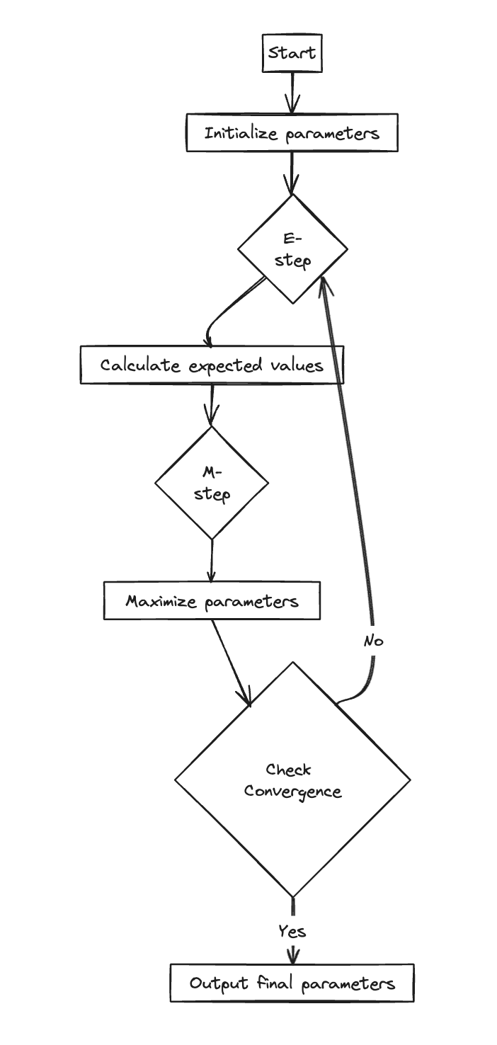
Therefor, we optimize it through a two-step process
- Expectation Step: Fix \(\theta\) to be \(\theta^{old}\), evaluate the posterior distribution of \(Z\) , i.e., because we know the form of the likelihood, we can calculate the posterior as long as a prior of \(Z\) is given. \[ P(Z = z | \theta^{old}, X) = \frac{P(Z|\theta^{old})P(X|Z,\theta^{old})}{P(X|\theta^{old})} = \frac{P(Z|\theta^{old})P(X|Z,\theta^{old})}{\sum_{z}P(Z|\theta^{old})P(X|\theta^{old})} \]
- Maximization Step: Maximize the likelihood \(P(X|\theta)\) but use the posterior \(P(Z|\theta^{old},X)\) in place of the prior \(P(Z|\theta)\), i.e., maximize \[ Q(\theta, \theta^{old}) = \sum_{z} P(Z|\theta^{old}, X)P(X|Z, \theta) \]
- Repeat the two steps until convergence.
We can interpret the EM algorithm by considering a decomposition of the likelihood, i.e., \[ \begin{aligned}\ln(p(X|\theta)) &= \mathcal{L}(q, \theta) + KL(q||p) \\&= \sum_{Z}q(Z)\ln(\frac{p(X, Z| \theta)}{q(Z)}) - \sum_{Z}q(Z)\ln(\frac{p(Z|\theta,X)}{q(Z)}) \\&= \sum_{Z}q(Z)\ln(p(X,Z|\theta)) - \sum_{Z}q(Z)\ln(p(Z|\theta, X)) \\&=\sum_{Z}q(Z)\ln(\frac{p(X,Z|\theta)}{p(Z|\theta, X)})\\&=\sum_{Z}q(Z)\ln(p(X|\theta)) \\&=\ln(p(X|\theta))\end{aligned} \] where \(q(Z)\) is an arbitrary prior of \(Z\).
This decomposition tells us that for given a fixed \(\theta\), the best prior \(q(Z)\) is found by letting it equal to the posterior \(p(Z|\theta, X)\), since it’s the only way to make the KL divergence 0. Also, for a fixed \(P(Z)\), we can obtain the best \(\theta\) by using maximal likelihood optimization.
Limitations
While the idea of EM is powerful, it is impractical in models where the evaluation of the posterior \(p(Z|\theta, X)\) is impossible (think multi-layer deep neural network with nonlinearity in between).
To make inference about \(Z\) in those cases, we need to resort to another powerful tool (Variational Inference).