EM in a nutshell
The idea behind EM is summarized as follows:
- Normally, in a learning problem, we are given a dataset $X$, we think of a model that capture the probability of the dataset $P(x)$, and the model is governed by a bunch of parameters $\theta$.
- What we do in machine learning (typically), is to solve for $\theta$ by optimizing for the likelihood of the data, given by
$$ P(X|\theta) $$
- one example would be logistic regression for multi-class classification, where
$$ P(X|\theta) = \prod_{n=1}^N \frac{\sum_{k=1}^K\exp(\theta^Tx_n)\cdot y_{nk}}{\sum_{k=1}^K\exp(\theta^Tx_n)} $$
-
To maximize the likelihood of the data, we typically take the log of the likelihood and maximize it using
- close-form solution (if available and dataset is small enough), e.g., linear regression
- gradient descent (if close-form solution is not available or dataset is too large)
-
However, there’re often cases where the distribution can’t be modeled so “simply”, meaning there’re more structure to the underlying distribution, where the distribution of $X$ is not only determined by $\theta$, but also by another set of random variables $Z$, one such example would be mixed gaussian where
$$ \begin{aligned}P(X|\theta) &= \sum_{z=k}^K P(X, Z|\theta) \&= \sum_{z=k}^KP(Z=z|\theta)P(X|Z=z, \theta) \&= \prod_{n=1}^N \sum_{z=k}^KP(z | \theta)P(x_n|Z = z, \theta) \&=\prod_{n=1}^N \sum_{z=k}^K \pi_{k}\mathcal{N}(x_n | \mu_z, \sigma_z)\end{aligned} $$
because there’s a sum inside the product, when taking the log of the likelihood, the close-form solution becomes very complex and hard to directly optimize for
-
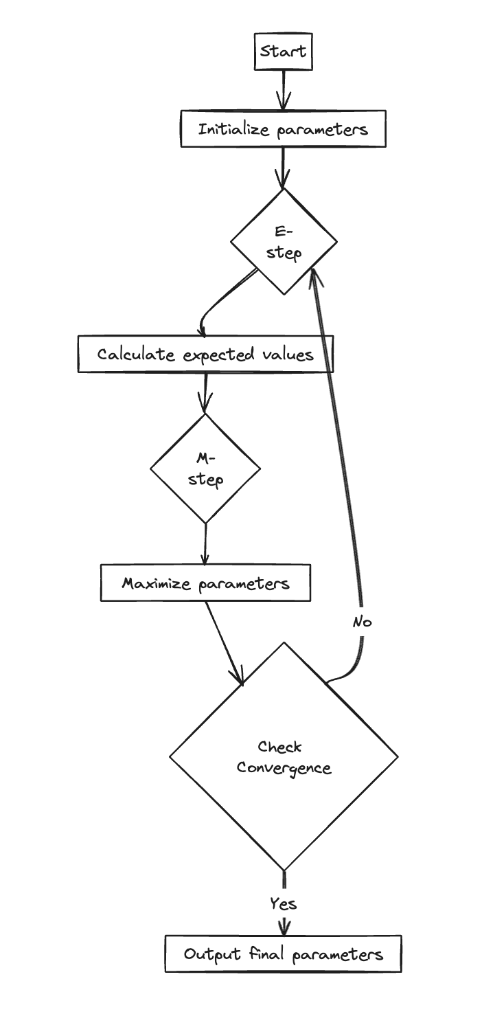
Therefor, we optimize it through a two-step process
- Expectation Step: Fix $\theta$ to be $\theta^{old}$, evaluate the posterior distribution of $Z$ , i.e., because we know the form of the likelihood, we can calculate the posterior as long as a prior of $Z$ is given.
$$ P(Z = z | \theta^{old}, X) = \frac{P(Z|\theta^{old})P(X|Z,\theta^{old})}{P(X|\theta^{old})} = \frac{P(Z|\theta^{old})P(X|Z,\theta^{old})}{\sum_{z}P(Z|\theta^{old})P(X|\theta^{old})} $$
- Maximization Step: Maximize the likelihood $P(X|\theta)$ but use the posterior $P(Z|\theta^{old},X)$ in place of the prior $P(Z|\theta)$, i.e., maximize
$$ Q(\theta, \theta^{old}) = \sum_{z} P(Z|\theta^{old}, X)P(X|Z, \theta) $$
- Repeat the above until convergence
-
We can interpret the EM algorithm by considering a decomposition of the likelihood, i.e.,
$$ \begin{aligned}\ln(p(X|\theta)) &= \mathcal{L}(q, \theta) + KL(q||p) \&= \sum_{Z}q(Z)\ln(\frac{p(X, Z| \theta)}{q(Z)}) - \sum_{Z}q(Z)\ln(\frac{p(Z|\theta,X)}{q(Z)}) \&= \sum_{Z}q(Z)\ln(p(X,Z|\theta)) - \sum_{Z}q(Z)\ln(p(Z|\theta, X)) \&=\sum_{Z}q(Z)\ln(\frac{p(X,Z|\theta)}{p(Z|\theta, X)})\&=\sum_{Z}q(Z)\ln(p(X|\theta)) \&=\ln(p(X|\theta))\end{aligned} $$
where $q(Z)$ is an arbitrary prior of $Z$.
This decomposition tells us that for given a fixed $\theta$, the best prior $q(Z)$ is found by letting it equal to the posterior $p(Z|\theta, X)$, since it’s the only way to make the KL divergence 0. Also, for a fixed $P(Z)$, we can obtain the best $\theta$ by using maximal likelihood optimization.
Limitations
While the idea of EM is powerful, it is impractical in models where the evaluation of the posterior $p(Z|\theta, X)$ is impossible (think multi-layer deep neural network with nonlinearity in between).
To make inference about $Z$ in those cases, we need to resort to another powerful tool (Variational Inference).